Winning systems: Analysing Handicap Chases – Variable Influence In his latest column for attheraces.com, Dr Peter May takes a closer look at numerous variables that influence handicap chase races.
Posted by Lydia Unwin on
ANALYSING HANDICAP CHASES – VARIABLE INFLUENCE
The conventional approach to race analysis requires the Analyst to evaluate various properties of each of the runners and then make a decision based on some form of weighted assessment of these values. Whilst the evaluation of the individual attributes is critical to the outcome of the method, the way these are combined into a single assessment of the runner’s chances of success is an equally crucial part of the calculation.
For example, a good recent run would be seen as a positive factor, whereas a significant rise in the handicap may be considered to be negative. These positives and negatives are then used to produce the forecast. However mentally combining these factors into a single assessment of chance of success is not easy, especially if the Race Analyst is not entirely sure of the level of significance of each attribute.
This article explores this area a little further and attempts to elicit the importance of some of the key factors used in such approaches.
With Autumn approaching it seems to be an appropriate time to focus on jumps racing, so the chosen race type for this article is handicap chases. To form the basis of the data, two years were chosen, and a third year, which does not form any part of the modelling process, was used for validation.
One method that can be used to identify the relationship between a specific attribute and the chance of success is to simply analyse historical data and generate a set of percentages for each value the attribute can take. So, if we wanted to know the relevance of a previous course win we could analyse the data and generate two proportions, one relating to the success rate of horse which had won previously at the track and the other for horses that have not been successful.
In this case, for handicap chases, these two figures would be remarkably similar suggesting limited importance, but for other factors there are significant differences. A linear regression model could also be used to determine the relative importance of each variable.
An alternative approach, and the one I have used many times, is to create a neural network model using the factors of interest and the race result as the outcome, or target variable. For this article I chose the following factors: Age of Runner, Course Absence, Weight Carried, Position on Last Run, and Last Race Price Ratio (LRPR).
All of these are well known and need no further explanation except for, perhaps, the final attribute.
The LRPR is simply the starting price of the horse on its last run divided by the number of runners in that race. Essentially this figure illustrates the degree of market confidence behind the horse on its last start, with a low figure suggesting a higher level of confidence.
The advantage of using this type of model to identify the importance of the variables is that it is immune to any correlation between the inputs, and it smoothes the data thus removing the outliers that may appear with a discrete model. The model was trained and then validated on a new set of data.
Overall, we would have expected a success rate of around 12%, however the model’s win rate was a reasonable 22%, which did equate to a small profit.
To generate the importance of the variables the weights of the model were examined and the following degrees of influence extracted: LRPP: 23%; Age 13%, Course Absence: 13%; Weight Carried: 13%; Position LTO: 13%; others factors in the model (for horses that did not complete on their last run) and the bias: 25%.
Consequently, the LRPR was the most influential input as far as the model was concerned with the other variables of similar importance to each other.
In order to provide a greater level of detail for each factor, various test data sets were assembled where the variable of interest was allowed to range across its possible values whilst the other factors remained constant at their median values.
These were interrogated by the model and the outputs recorded. Since the target variable was a binary representation of the finishing position (1=win, 0=lost) a high value suggests a greater chance of success.
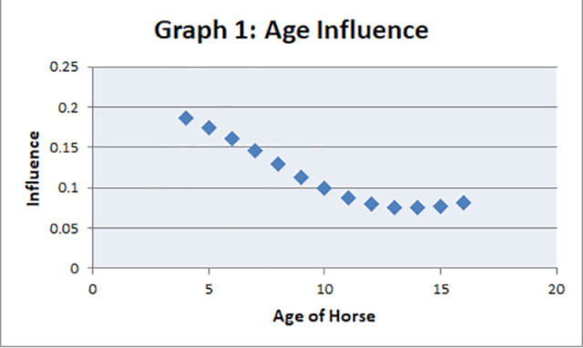
Graph 1 shows the model’s output associated with the Age variable. From the graph we can immediately see that younger horses produce a higher output with the level decreasing then flattening out for those aged 11 and over. This would seem reasonable and not many Analysts would disagree with the finding.
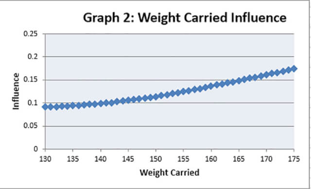
Weight Carried (Graph 2) shows an almost linear trend with the higher weights being favoured
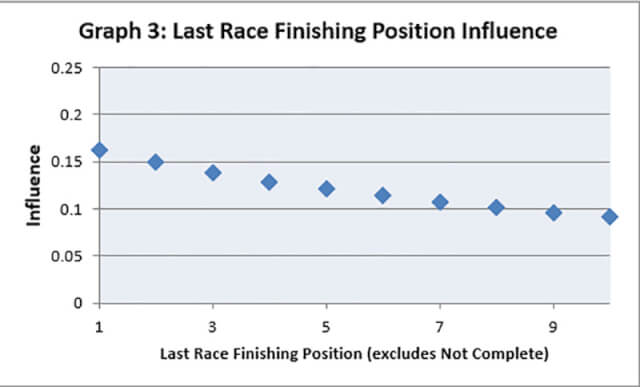
which is similar to Position Last time (Graph 3) although the slope is in the opposite direction.
The LRPR graph (Graph 4) is possibly the most interesting. To form the graph the LRPR figure was ranked for each race with the smallest figure ranked as 1.
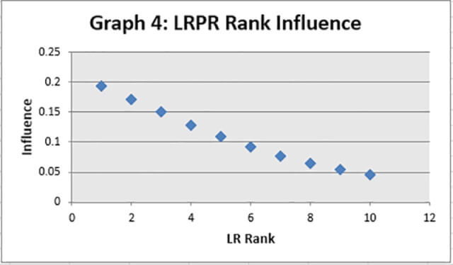
The graph shows a steep decline (steep is always good for type of analysis) from a high figure around 0.19 to a low of 0.05. This demonstrates the importance of the attribute (for instance it is more influential than the position last time out factor) and thus how useful it is in any forecasting model.
Finally Graph 5 presents the Course Absence factor, the form of which may be a little surprising. As can been seen the line is almost flat suggesting that this attribute has no overall impact on the model. In some models this could be due to high correlation with other factors, but given those chosen for this model this is clearly not the case.
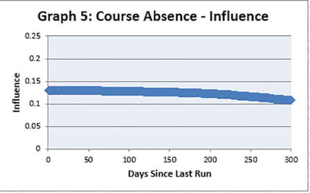
So why is this graph so flat when the overall level of influence is as high as some of the other factors?
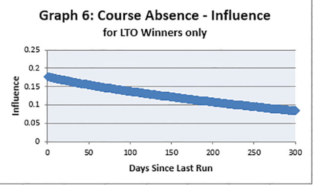
Well, the graph shows the influence of the Course Absence factor for an average runner, in other words a horse which has average scores for the other variables. But for some runners this variable has much more impact (see Graph 6).
For models like linear regression the impact each variable has on the output remains constant across runners. In other words, and win last time out will make the same contribution to the output regardless of the other attributes of the runner. However, a neural network does not consider each variable in isolation, so the impact will not just depend on the attribute but the values of the other variables associated with the horse.
For average runners the graph for Course Absence maybe flat, but if we change one, or more, of the other variables we find a more interesting relationship.
In Graph 6 the outputs for the Course Absence attribute have been presented not for average runners, but for those horses which won their last race. The slope is now steeper, but what does it suggest? Essentially a previous race win is more important if it happened recently, again that would be a logical assessment.
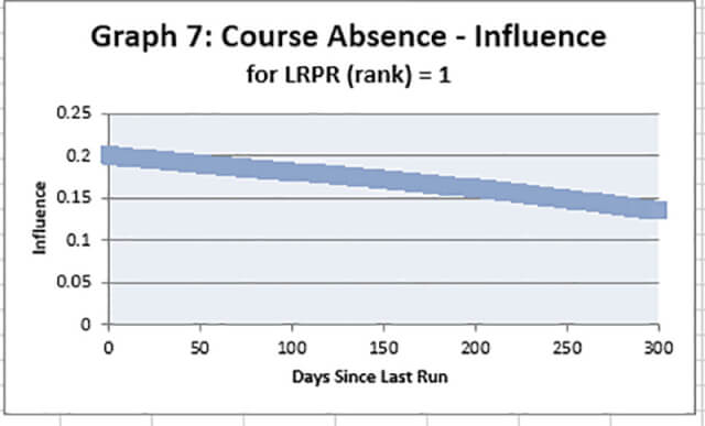
Graph 7 shows the same relationship but for horses which are ranked top for the LRPR variable. On its own the LRPR variable produced a model output of around 0.19 when its value was 1, however when looked in relation to the Course Absence variable we can see that this figure drops to 0.13 as the number of days off the track increases.
So, whilst models like this can be used to confirm our understanding of the importance of each factor, they also show that it can be dangerous to treat these factors in isolation and a more holistic view should be adopted if possible.
